Graphical abstract
1
Fixed threshold
FixMatch, UniMatch, UniMatch V2 (τ = 0.95)
Slums get the fewest pseudo-labels.
2
Prevalence-scaled
FreeMatch class term (slum threshold below 0.49)
Over-corrects and over-predicts slums.
3
Confidence-scaled
Ours: class term from per-class confidence
Tracks the labels. No new hyperparameter.
TL;DRA fixed pseudo-label threshold starves the rare slum class, and prevalence-scaled thresholds over-correct. Scaling the threshold by per-class confidence raises slum IoU in 49 of 54 settings across three cities, two sensors and three methods.
Abstract
Maps of informal settlements support urban planning, but pixel-level labels exist for few cities. Semi-supervised segmentation methods such as FixMatch, UniMatch and UniMatch V2 train on pseudo-labels and keep a pixel only if its confidence exceeds a fixed threshold. Slums are the minority class and the model is less confident on them, so this threshold discards slum pixels far more often than background pixels, while class-adaptive thresholds that scale with class prevalence let the model over-predict slums. We keep the self-adaptive threshold of FreeMatch but compute its class term from the mean confidence of the pixels predicted as each class, which adds no hyperparameter. We evaluate it on a new annotation of the informal settlements of Lahore and on public labels of Karachi and Mumbai, with 0.5 m very-high-resolution and 10 m Sentinel-2 imagery and spatial splits. Across three methods, two sensors, three cities and three label budgets, the threshold raises the slum intersection over union in 49 of 54 settings, by 3.65 points on average (95% confidence interval 2.21 to 5.33), most for FixMatch, at 10% labels and on Sentinel-2.
1 Introduction
More than half of the world’s population lives in cities, a share the United Nations expects to reach two thirds by 2050 [1]. In many low- and middle-income countries, part of this growth becomes informal settlements, characterized by insecure tenure, inadequate services, and unplanned housing [2]. In Pakistan, these settlements are largely missing from official records, and a UNICEF survey of ten cities found worse health, housing, and education in them than in the cities overall [3]. Planning and service delivery need settlement maps, which ground surveys cannot produce at city scale.
Satellite imagery can. Informal settlements have been mapped with built-up indices [4], texture features [5], object-based classifiers [6], and deep segmentation networks on very-high-resolution (VHR) imagery [7, 8]. These networks need pixel-level labels, which take local knowledge to draw and exist for few cities. VHR mosaics also usually cannot be redistributed, whereas Sentinel-2 data [9] can, at 10 m resolution [10].
Semi-supervised learning also trains on unlabelled images, and in remote sensing segmentation it has used transformation consistency [11], contrastive learning [12], and label propagation [13]. FixMatch [14], UniMatch [15], and UniMatch V2 [16] predict pseudo-labels on weakly augmented images, train on strongly augmented versions, and keep a pixel only if its confidence exceeds a fixed threshold, usually 0.95. This value was tuned on natural-image benchmarks with roughly balanced classes, whereas pseudo-labels on imbalanced aerial images favour the larger classes [17, 18]. Slums cover few pixels and the teacher is less confident on them, so the fixed threshold discards a larger share of slum than of background pixels (Section 3.2).
Class-adaptive thresholds [19, 20, 17] lower the threshold for classes that the model learns slowly, also in remote sensing segmentation [21], and percentile-based selection [22] ranks pixels instead of thresholding them. FreeMatch [20] scales each class threshold by the mean predicted probability of the class, which also tracks how often the class occurs. With one rare class out of two, this keeps the slum threshold below 0.5, and the teacher labels a growing share of pixels as slum (Section 3.4).
We keep the self-adaptive threshold of FreeMatch but compute its class term from the mean confidence of the pixels predicted as each class, following Chen et al. [23]. It adds no hyperparameter and replaces only the mask of the unsupervised loss, so it applies to all three methods unchanged. We evaluate it on a new annotation of the Katchi Abadis (informal settlements) of Lahore, derived from government records, and on public Karachi and Mumbai labels, built with an open pipeline [24] for VHR and Sentinel-2 imagery and split by location. Across three methods, three cities, two sensors, and three label budgets, it raises the intersection over union (IoU) of the slum class in 49 of 54 settings, by 3.65 points on average (95% CI 2.21 to 5.33).
2 Dataset
2.1 Labels
The Lahore labels are new. Two annotators independently delineated the 266 settlements in the records of the Katchi Abadis Directorate of Lahore on Google Earth imagery [25] and resolved their disagreements in a joint review. The Karachi labels are the Katchi Abadi map of Karachi Cartography [26], with 529 polygons, of which we treat the four larger than 500 ha as unlabelled, since they are far larger than any settlement elsewhere. The Mumbai labels are the slum cluster map of the Slum Rehabilitation Authority [27], with 2,541 polygons. In Lahore, informal and planned neighbourhoods can share the same dense built-up texture (Fig. 1), so appearance alone does not separate them.
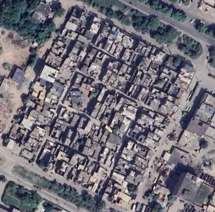 Zia Colony · informal
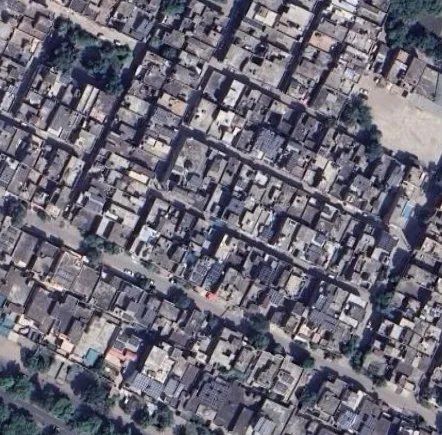 Township · planned
Zia Colony, an informal settlement [28] (left), and Township, a planned neighbourhood (right), in Lahore. Both show the same dense built-up texture. Google Earth imagery [ 25].
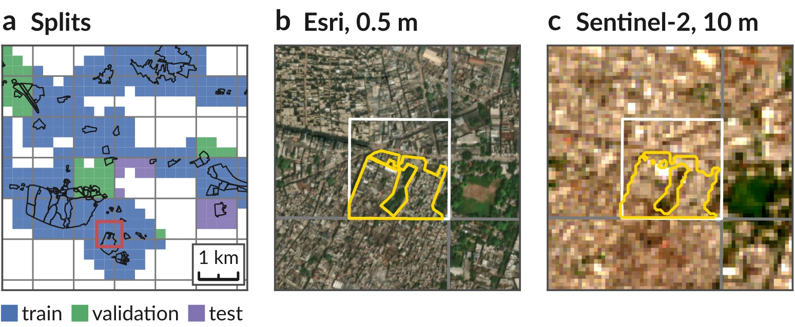
Spatial splits and one tile in both sensors. (a) Lahore tiles by split, with the blocks of 2048×2048 pixels (grey) and the settlement polygons (black). (b) Esri and (c) Sentinel-2 views of the 640 m window marked in red, with the labelled tile (white) and its slum label (yellow).
2.2 Imagery
New labels. Two annotators drew all 266 Lahore settlements by hand from government records.
We build the datasets with mapcv [24], which reads Esri World Imagery [29] at zoom level 18 within 250 m of the polygons and cuts it into non-overlapping RGB tiles of pixels, about 0.5 m per pixel. A pixel is slum if its centre lies inside a polygon and background otherwise, so background means outside the mapped settlements, not verified formal housing. Tiles with more than 5% missing imagery are discarded, and in Karachi also tiles that are more than half unlabelled, which leaves 792 of 1,850 tiles. For Sentinel-2 we use one L2A acquisition per city [9] from Earth Search [30] with less than 0.01% cloud cover, merging the two granules of the pass. We use the ten bands at 10 and 20 m, with the 20 m bands repeated to 10 m, zero the pixels classified as cloud, cirrus, or cloud shadow, and rasterize the labels at 10 m. For every VHR tile we cut a window (640 m) centred on it, label only the 26 to 29 pixels on a side that lie inside the tile, and use the rest as context (Fig. 2c). Window pixels in tiles of another split are set to zero, 7 to 9% of a window on average, so that no training window contains validation or test ground. Each window takes the split of its tile, so the two sensors share the splits and label budgets of Table 1. Esri imagery and the Karachi map may not be redistributed, so we release the configurations and scene identifiers that rebuild the datasets instead of the images and masks. (code: https://github.com/tahamukhtar20/Slum-i)
| Statistic | Lahore | Karachi | Mumbai |
|---|---|---|---|
| Area (km²) | |||
| Labelled | 136.3 | 55.0 | 297.1 |
| Slum | 24.4 | 12.9 | 33.4 |
| Number of tiles | |||
| Total | 2,006 | 792 | 3,559 |
| Training | 1,534 | 633 | 2,715 |
| labelled at 10% | 154 | 60 | 272 |
| labelled at 20% | 307 | 123 | 543 |
| labelled at 30% | 461 | 185 | 815 |
| Validation | 171 | 66 | 310 |
| Test | 301 | 93 | 534 |
| Slum pixels (%) | |||
| Training | 17.1 | 23.6 | 11.4 |
| Validation | 11.5 | 28.9 | 9.8 |
| Test | 25.6 | 18.3 | 11.3 |
2.3 Spatial Splits
Neighbouring tiles look alike, so random tile splits place near copies of test tiles in the training set and overestimate accuracy [31]. mapcv therefore assigns whole blocks of VHR pixels, 1.0 to 1.2 km on a side, to the test and validation sets (Fig. 2a), with targets of 15% and 10% of the tiles, and the remaining tiles form the training set. The labelled subsets contain 10%, 20%, and 30% of the training tiles and are nested, and the other training tiles form the unlabelled set. Because the splits follow location, their slum shares differ, in Lahore from 11.5% in validation to 25.6% in test.
3 Method
3.1 Pseudo-Labelling Baselines
The three baselines share one teacher–student scheme. For each pixel of a weakly augmented unlabelled image, a teacher predicts class probabilities , with confidence and pseudo-label . A student learns on strongly augmented views of the image, and only confident pixels enter the unsupervised loss,
where the sum runs over the valid pixels of the batch, is the student prediction and . FixMatch [14] uses the student as its own teacher. UniMatch [15] adds a second strong view and a feature-perturbation stream. UniMatch V2 [16] uses a DINOv2 encoder [32], an EMA teacher and complementary feature dropout. The training loss adds to the supervised cross-entropy.
3.2 Class Bias in the Pseudo-Labels
Slums are the minority class in every city and their boundaries are ambiguous, so the teacher is less confident on them and a single threshold drops them more often. In diagnostic runs of UniMatch V2 at 10% labels, after ten epochs the fixed threshold keeps 43–70% of the pixels predicted as slum but 90–96% of those predicted as background. The class of interest thus receives the least supervision early in training, when pseudo-labels shape the student most.
3.3 Adaptive Threshold
We adopt the self-adaptive threshold of FreeMatch [20], in which each class threshold is the global threshold scaled by a normalised class term. FreeMatch computes this term from the mean class probability, which also scales with class prevalence. Following the class-level confidence of Chen et al. [23], we instead use the mean confidence of the pixels predicted as each class, and we omit the fairness loss (Fig. 3).
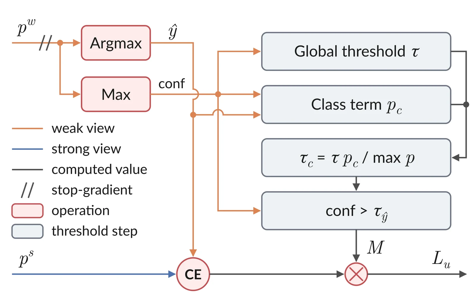
Adaptive pseudo-label threshold. The global threshold is an exponential moving average (EMA) of the mean confidence of all pixels, and the class term is an EMA of the mean confidence of the pixels predicted as class . The mask keeps a pixel if its confidence exceeds the threshold of its predicted class , and it is multiplied with the pixel-wise cross-entropy (CE) loss to give the unsupervised loss .
At step , the teacher outputs on the unlabelled batch update the global threshold and the class term,
where is the number of valid pixels predicted as class and as in FreeMatch. Both terms start at , and a class absent from the batch keeps its previous value. The threshold of class is
and the mask in (1) becomes . The most confident class keeps the global threshold, and the others are lowered in proportion to their confidence gap. The mask replaces the fixed threshold in every unsupervised stream of each baseline, and no hyperparameter is added. We write Ours (X) for baseline X with this threshold.
3.4 Effect on the Pseudo-Labels
Because the class term follows confidence rather than prevalence, the slum threshold starts below the background threshold (0.74 against 0.87 in Lahore after ten epochs) and rises to 0.96–0.97 as the teacher becomes confident on slums. With the FreeMatch term, the slum threshold stays below 0.49, and the share of pixels the teacher labels as slum grows from 11–15% under the fixed threshold to 22–31% by the last epoch. Our threshold keeps this share at 12–18%.
4 Experiments and Results
4.1 Setup
No checkpoint picking. Every run is scored after its last epoch, so a lucky early checkpoint cannot inflate a number.
FixMatch and UniMatch use DeepLabV3+ [33] with an ImageNet-pretrained ResNet-101 [34], trained for 80 epochs with SGD at a learning rate of 0.02 on crops. UniMatch V2 uses a DPT head [35] on DINOv2-S [32], fine-tuned for 60 epochs with AdamW at a learning rate of for the encoder and 40 times higher for the head, on crops. Each step uses 8 labelled and 8 unlabelled images. For Sentinel-2, the first layer takes the ten bands and the windows are resized to pixels. The supervised baselines use the same two networks and are trained on the labelled tiles only, at 10, 20, 30 and 100% of the training set. All other hyperparameters follow the official implementations and are shared by all cities, sensors and methods. Every configuration is run with five seeds and scored on the test set after the last epoch, without checkpoint selection. We report the slum IoU as the main metric and the mean IoU (mIoU) over slum and background.
4.2 Qualitative Results
Fig. 4 shows one test tile per city at 10% labels. In Lahore, both baselines miss large parts of the slum, and our threshold recovers part of it, most clearly for FixMatch. In Karachi, FixMatch and UniMatch mark a large non-slum area as slum. Our threshold removes most of it for UniMatch, while for FixMatch it misses more of the slum strip and adds false slum pixels at the bottom of the tile. In Mumbai, all models give similar maps.
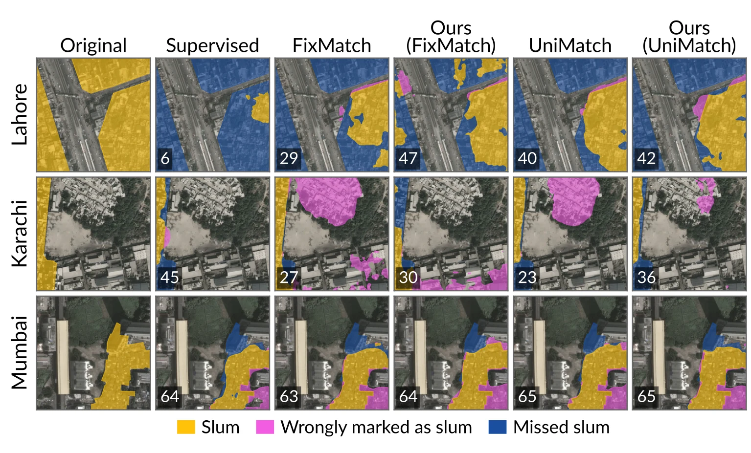
Qualitative comparison at 10% labels (Esri imagery). Original shows the labelled slums. In the other columns, gold marks slums each model found, magenta marks areas wrongly marked as slum, and blue marks missed slums. Numbers give the slum IoU of each tile.
4.3 Results
Where it fails. Karachi with Sentinel-2 is hard for everyone. The section below says exactly how.
Table 2 lists all results. Across the 54 settings of three baselines, two sensors, three cities and three label budgets, our threshold raises the mean slum IoU in 49, and an Ours row has the best slum IoU in 33 of the 36 backbone blocks. The mean paired change is slum IoU (95% bootstrap interval 2.21 to 5.33, Wilcoxon signed-rank ) and mIoU (0.13 to 1.61, ). Gains are largest where the baseline is weakest, with slum IoU for FixMatch, at 10% labels and on Sentinel-2 against on Esri, and smallest in Mumbai (), where the baselines are already close to full supervision. In 13 settings a model with our threshold exceeds the supervised model of the same backbone trained on all labels in both metrics, against 5 for the baselines, for example Ours (FixMatch) at 30% labels in Lahore on Esri imagery (59.8 against 56.8 slum IoU).
| City | Lahore | Karachi | Mumbai | |||||||||
|---|---|---|---|---|---|---|---|---|---|---|---|---|
| Sensor | Esri | Sentinel-2 | Esri | Sentinel-2 | Esri | Sentinel-2 | ||||||
| Method | mIoU | Slum | mIoU | Slum | mIoU | Slum | mIoU | Slum | mIoU | Slum | mIoU | Slum |
| 10% labels | ||||||||||||
| Supervised (R101) | 52.9±4.6 | 28.0±8.3 | 53.7±4.2 | 32.6±6.4 | 53.3±2.1 | 27.0±3.3 | 47.9±2.1 | 18.4±3.3 | 78.7±0.1 | 62.8±0.2 | 75.3±0.5 | 56.8±1.1 |
| FixMatch | 64.7±4.0 | 48.3±6.4 | 55.9±3.1 | 34.0±5.0 | 48.0±3.5 | 22.0±12.7 | 40.8±0.1 | 0.1±0.1 | 79.0±0.7 | 63.5±1.1 | 74.4±0.6 | 55.1±1.2 |
| Ours (FixMatch) | 69.5±1.8 | 56.2±2.5 | 63.5±2.5 | 52.1±2.8 | 51.9±4.9 | 32.6±4.7 | 28.5±11.6 | 13.4±11.2 | 79.2±0.5 | 64.2±0.7 | 71.9±1.9 | 52.4±2.8 |
| UniMatch | 64.7±3.3 | 48.4±5.5 | 61.7±2.6 | 45.3±4.4 | 53.6±1.6 | 31.2±2.0 | 45.5±1.7 | 13.3±3.7 | 79.3±0.2 | 63.9±0.4 | 75.2±1.4 | 56.7±2.5 |
| Ours (UniMatch) | 67.1±1.2 | 52.5±1.8 | 64.0±2.9 | 49.0±4.6 | 51.5±4.6 | 32.8±3.8 | 46.5±2.0 | 16.2±5.6 | 79.5±0.1 | 64.4±0.2 | 75.9±1.2 | 57.9±2.1 |
| Supervised (DINOv2) | 64.0±0.9 | 46.5±1.4 | 58.4±3.1 | 40.3±4.7 | 61.2±2.2 | 37.5±3.8 | 49.8±1.0 | 20.0±1.6 | 79.4±0.3 | 64.0±0.6 | 76.4±0.2 | 58.8±0.4 |
| UniMatch V2 | 61.1±2.0 | 41.8±2.9 | 65.3±2.7 | 50.6±4.3 | 65.8±1.2 | 45.6±1.9 | 49.5±1.7 | 20.0±2.9 | 80.9±0.2 | 66.6±0.3 | 78.0±0.4 | 61.6±0.7 |
| Ours (UniMatch V2) | 65.9±2.2 | 50.7±3.3 | 65.7±2.0 | 53.5±2.9 | 67.9±1.5 | 49.9±2.8 | 51.6±2.7 | 23.8±5.7 | 80.8±0.6 | 66.6±0.9 | 78.0±0.1 | 61.9±0.3 |
| 20% labels | ||||||||||||
| Supervised (R101) | 58.8±5.8 | 38.0±9.9 | 56.4±2.9 | 35.8±5.2 | 60.2±0.9 | 37.5±1.7 | 50.7±1.2 | 24.6±2.5 | 79.1±0.1 | 63.4±0.2 | 75.5±0.7 | 57.1±1.2 |
| FixMatch | 70.0±0.6 | 56.0±1.0 | 56.6±4.7 | 35.2±7.9 | 62.6±3.6 | 43.5±6.7 | 41.3±0.9 | 1.3±1.5 | 80.4±0.5 | 65.8±0.7 | 75.7±0.9 | 57.4±1.7 |
| Ours (FixMatch) | 71.1±2.5 | 58.3±3.9 | 64.2±0.7 | 49.5±1.4 | 60.3±3.8 | 44.2±3.6 | 42.2±6.2 | 28.4±3.0 | 80.7±0.4 | 66.4±0.7 | 75.6±1.0 | 57.7±1.6 |
| UniMatch | 70.2±2.1 | 56.6±3.2 | 60.9±4.3 | 43.2±6.5 | 63.8±3.3 | 45.6±4.5 | 49.5±2.3 | 22.1±5.3 | 80.2±0.1 | 65.5±0.2 | 75.7±0.7 | 57.8±1.3 |
| Ours (UniMatch) | 69.1±1.1 | 54.9±1.8 | 62.9±1.1 | 46.8±1.8 | 65.2±3.2 | 48.5±3.3 | 50.6±1.5 | 26.1±4.3 | 80.4±0.1 | 65.9±0.2 | 76.5±0.7 | 59.1±1.2 |
| Supervised (DINOv2) | 67.0±1.3 | 51.1±2.0 | 62.4±1.6 | 45.2±2.2 | 68.6±0.5 | 51.1±0.9 | 54.5±2.6 | 28.7±3.9 | 80.5±0.3 | 65.9±0.5 | 77.3±0.5 | 60.4±0.9 |
| UniMatch V2 | 67.6±2.7 | 51.8±4.2 | 64.6±1.2 | 48.6±2.4 | 69.3±1.1 | 52.5±1.6 | 58.4±1.5 | 35.6±2.1 | 81.5±0.3 | 67.7±0.6 | 78.4±0.2 | 62.3±0.4 |
| Ours (UniMatch V2) | 71.4±2.5 | 58.5±3.9 | 66.1±1.3 | 52.4±1.5 | 69.4±0.8 | 53.1±1.1 | 56.1±3.0 | 31.9±6.4 | 81.5±0.1 | 67.7±0.2 | 78.8±0.4 | 63.0±0.7 |
| 30% labels | ||||||||||||
| Supervised (R101) | 62.7±1.6 | 44.3±2.8 | 59.4±3.6 | 40.7±5.6 | 59.6±1.3 | 35.6±2.5 | 52.4±3.0 | 26.9±5.4 | 79.7±0.5 | 64.5±1.0 | 76.4±0.5 | 58.8±1.0 |
| FixMatch | 71.7±2.1 | 58.5±3.5 | 61.1±1.7 | 42.7±2.8 | 63.0±2.4 | 41.1±3.8 | 45.2±3.6 | 10.3±8.4 | 80.8±0.4 | 66.4±0.8 | 76.1±0.7 | 58.0±1.2 |
| Ours (FixMatch) | 72.3±1.6 | 59.8±2.3 | 63.5±2.2 | 48.7±2.7 | 66.0±1.5 | 49.0±1.9 | 51.7±1.8 | 33.2±1.5 | 81.2±0.3 | 67.3±0.5 | 76.5±0.7 | 58.9±1.2 |
| UniMatch | 71.3±1.9 | 58.1±3.0 | 61.6±1.8 | 43.9±3.1 | 63.6±2.5 | 44.2±4.0 | 51.4±3.1 | 24.6±6.1 | 80.7±0.2 | 66.2±0.4 | 76.7±0.6 | 59.2±1.1 |
| Ours (UniMatch) | 69.5±2.8 | 55.1±4.4 | 62.2±1.6 | 44.8±2.9 | 64.4±3.1 | 45.1±5.2 | 51.9±2.7 | 27.2±4.9 | 81.0±0.1 | 66.9±0.1 | 76.8±0.2 | 59.5±0.4 |
| Supervised (DINOv2) | 67.2±1.7 | 51.3±2.5 | 59.9±1.8 | 40.6±2.9 | 67.4±1.9 | 48.6±3.0 | 54.5±2.1 | 28.5±3.3 | 81.0±0.1 | 66.8±0.2 | 78.1±0.6 | 61.7±1.0 |
| UniMatch V2 | 67.1±1.3 | 51.2±1.9 | 66.7±2.5 | 51.6±4.1 | 67.9±1.8 | 49.3±2.7 | 57.2±3.0 | 33.0±5.4 | 81.6±0.3 | 67.8±0.5 | 78.9±0.3 | 63.2±0.5 |
| Ours (UniMatch V2) | 70.0±1.5 | 55.9±2.3 | 67.1±1.5 | 53.4±2.4 | 67.9±1.0 | 49.8±1.2 | 57.4±2.2 | 33.6±3.7 | 81.8±0.3 | 68.2±0.6 | 79.1±0.2 | 63.6±0.3 |
| 100% labels | ||||||||||||
| Supervised (R101) | 70.9±1.2 | 56.8±2.2 | 63.3±1.1 | 47.2±1.7 | 63.1±1.0 | 41.2±1.8 | 52.2±3.2 | 26.9±5.3 | 81.5±0.2 | 67.6±0.4 | 77.7±0.5 | 61.0±1.0 |
| Supervised (DINOv2) | 71.7±0.7 | 58.6±1.3 | 69.1±0.4 | 55.2±0.6 | 67.8±1.6 | 49.6±2.4 | 59.3±2.6 | 36.7±4.5 | 82.1±0.3 | 68.8±0.5 | 78.9±0.2 | 63.2±0.4 |
The slum IoU drops in five settings, by at most 3.8 points, namely UniMatch on Lahore Esri at 20 and 30%, UniMatch V2 on Mumbai Esri at 10% and on Karachi Sentinel-2 at 20%, and FixMatch on Mumbai Sentinel-2 at 10%. Only the last is significant per setting (mIoU , paired -test ), where the model drifts towards over-predicting slums late in training. On Karachi Sentinel-2, the hardest setting, FixMatch collapses to background in every seed at 10 and 20% labels (slum IoU below 4). Our threshold avoids the collapse at 20%, with a slum IoU of 25 to 33 in every seed, but over-predicts slums. At 10% two seeds still collapse and three over-predict, and the supervised model keeps the best mIoU of this block.
5 Conclusion
A fixed confidence threshold gives the minority slum class the fewest pseudo-labels, and a threshold scaled by class prevalence over-corrects towards slums. Computing the class term of the FreeMatch threshold from class confidence instead raises the slum IoU of three semi-supervised methods in 49 of 54 settings across three cities and two sensors, with no new hyperparameter. The gain is small in Mumbai, and on Karachi Sentinel-2 the threshold avoids the collapse of FixMatch but over-predicts slums. Each city has one acquisition per sensor, and background means outside the mapped settlements, so omissions in the source maps count as model errors.
References
- [1]United Nations, Department of Economic and Social Affairs, Population Division, “World Urbanization Prospects 2025: Summary of Results”, United Nations, 2025. source
- [2]United Nations Human Settlements Programme (UN-Habitat), “Habitat III Issue Papers 22: Informal Settlements”, United Nations, 2015. source
- [3]United Nations Children's Fund (UNICEF), “Coverage Survey in Slums/Underserved Areas of 10 Largest Cities of Pakistan”, UNICEF Pakistan, 2020. source
- [4]Y. Zha, J. Gao and S. Ni, “Use of normalized difference built-up index in automatically mapping urban areas from TM imagery”, Int. J. Remote Sens., 2003. source
- [5]M. Kuffer, K. Pfeffer, R. Sliuzas and I. Baud, “Extraction of Slum Areas From VHR Imagery Using GLCM Variance”, IEEE J. Sel. Topics Appl. Earth Observ. Remote Sens., 2016. source
- [6]K. G. Alrasheedi, A. Dewan and A. El-Mowafy, “Combining local knowledge with object-based machine learning techniques for extracting informal settlements from very high-resolution satellite data”, Earth Systems and Environment, 2024. source
- [7]C. Persello and A. Stein, “Deep Fully Convolutional Networks for the Detection of Informal Settlements in VHR Images”, IEEE Geosci. Remote Sens. Lett., 2017. source
- [8]R. Fan, F. Li, W. Han, J. Yan, J. Li and L. Wang, “Fine-Scale Urban Informal Settlements Mapping by Fusing Remote Sensing Images and Building Data via a Transformer-Based Multimodal Fusion Network”, IEEE Trans. Geosci. Remote Sens., 2022. source
- [9]M. Drusch et al., “Sentinel-2: ESA's Optical High-Resolution Mission for GMES Operational Services”, Remote Sens. Environ., 2012. source
- [10]S. Gxokwe and T. Dube, “Using cloud computing techniques to map the geographic extent of informal settlements in the greater Cape Town Metropolitan Area”, Remote Sens. Appl.: Soc. Environ., 2024. source
- [11]B. Zhang et al., “Semi-Supervised Deep Learning via Transformation Consistency Regularization for Remote Sensing Image Semantic Segmentation”, IEEE J. Sel. Topics Appl. Earth Observ. Remote Sens., 2023. source
- [12]J. Wang, S. Chen, C. H. Q. Ding, J. Tang and B. Luo, “Semi-Supervised Semantic Segmentation of Remote Sensing Images With Iterative Contrastive Network”, IEEE Geosci. Remote Sens. Lett., 2022. source
- [13]Z. Yang et al., “Label Propagation and Contrastive Regularization for Semisupervised Semantic Segmentation of Remote Sensing Images”, IEEE Trans. Geosci. Remote Sens., 2023. source
- [14]K. Sohn et al., “FixMatch: simplifying semi-supervised learning with consistency and confidence”, Proc. Adv. Neural Inf. Process. Syst. (NeurIPS), 2020.
- [15]L. Yang, L. Qi, L. Feng, W. Zhang and Y. Shi, “Revisiting Weak-to-Strong Consistency in Semi-Supervised Semantic Segmentation”, Proc. IEEE/CVF Conf. Comput. Vis. Pattern Recognit. (CVPR), 2023. source
- [16]L. Yang, Z. Zhao and H. Zhao, “UniMatch V2: Pushing the Limit of Semi-Supervised Semantic Segmentation”, IEEE Trans. Pattern Anal. Mach. Intell., 2025. source
- [17]L. Guo and Y. Li, “Class-Imbalanced Semi-Supervised Learning with Adaptive Thresholding”, Proc. Int. Conf. Mach. Learn. (ICML), 2022.
- [18]K. Nogueira, M. M. Faita-Pinheiro, A. P. M. Ramos, W. N. Goncalves, J. M. Junior and J. A. dos Santos, “Prototypical Contrastive Network for Imbalanced Aerial Image Segmentation”, Proc. IEEE/CVF Winter Conf. Appl. Comput. Vis. (WACV), 2024. source
- [19]B. Zhang et al., “FlexMatch: Boosting Semi-Supervised Learning with Curriculum Pseudo Labeling”, Proc. Adv. Neural Inf. Process. Syst. (NeurIPS), 2021.
- [20]Y. Wang et al., “FreeMatch: Self-adaptive Thresholding for Semi-supervised Learning”, Proc. Int. Conf. Learn. Represent. (ICLR), 2023.
- [21]S. Wang, C. Su and X. Zhang, “A Class-Aware Semi-Supervised Framework for Semantic Segmentation of High-Resolution Remote Sensing Imagery”, IEEE J. Sel. Topics Appl. Earth Observ. Remote Sens., 2025. source
- [22]Y. Wang et al., “Semi-Supervised Semantic Segmentation Using Unreliable Pseudo-Labels”, Proc. IEEE/CVF Conf. Comput. Vis. Pattern Recognit. (CVPR), 2022.
- [23]Z. Chen, L. Jing, L. Yang, Y. Li and B. Li, “Class-Level Confidence Based 3D Semi-Supervised Learning”, Proc. IEEE/CVF Winter Conf. Appl. Comput. Vis. (WACV), 2023.
- [24]M. T. Mukhtar, “mapcv: Computer-Vision Datasets from Map Imagery and Geospatial Labels”, Zenodo, 2026. source
- [25]Google, “Google Earth”, Web application, 2026. source
- [26]Karachi Cartography, “Katchi Abadi Map”, 2023.
- [27]Slum Rehabilitation Authority, Mumbai, “Mumbai - Slum Cluster Map”, 2015.
- [28]M. M. Arif, O. Devisch and Y. Schoonjans, “Examining the Intricacies and Perpetual Issues in Urban Informal Settlements: Lessons from Two Case Studies of Informal Settlements in Lahore, Pakistan”, Journal of Art, Architecture and Built Environment, 2023.
- [29]Esri, “World Imagery”, ArcGIS Online basemap, 2026. source
- [30]Element 84, “Earth Search: STAC API for Sentinel-2 L2A Cloud-Optimized GeoTIFFs on AWS”, 2026.
- [31]D. R. Roberts et al., “Cross-Validation Strategies for Data with Temporal, Spatial, Hierarchical, or Phylogenetic Structure”, Ecography, 2017. source
- [32]M. Oquab et al., “DINOv2: Learning Robust Visual Features without Supervision”, Trans. Mach. Learn. Res., 2024.
- [33]L.-C. Chen, Y. Zhu, G. Papandreou, F. Schroff and H. Adam, “Encoder-Decoder with Atrous Separable Convolution for Semantic Image Segmentation”, Proc. Eur. Conf. Comput. Vis. (ECCV), 2018.
- [34]K. He, X. Zhang, S. Ren and J. Sun, “Deep Residual Learning for Image Recognition”, Proc. IEEE Conf. Comput. Vis. Pattern Recognit. (CVPR), 2016. source
- [35]R. Ranftl, A. Bochkovskiy and V. Koltun, “Vision Transformers for Dense Prediction”, Proc. IEEE/CVF Int. Conf. Comput. Vis. (ICCV), 2021. source
Citation
@misc{mukhtar2026slumi,
  title         = {SLUM-i: Semi-Supervised Learning for Urban Mapping of Informal Settlements},
  author        = {Muhammad Taha Mukhtar and Syed Musa Ali Kazmi and Khola Naseem and Muhammad Ali Chattha and Andreas Dengel and Sheraz Ahmed and Muhammad Naseer Bajwa and Muhammad Imran Malik},
  year          = {2026},
  eprint        = {2602.04525},
  archivePrefix = {arXiv},
  primaryClass  = {cs.CV},
  url           = {https://arxiv.org/abs/2602.04525}
}